How to value a stock in Stoxa

Find the company

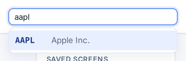
Type a ticker or company name into the search ticker or company… box at the top right of every page. Pick a result with the mouse or the arrow keys and Enter to open its company page.

Read the company page

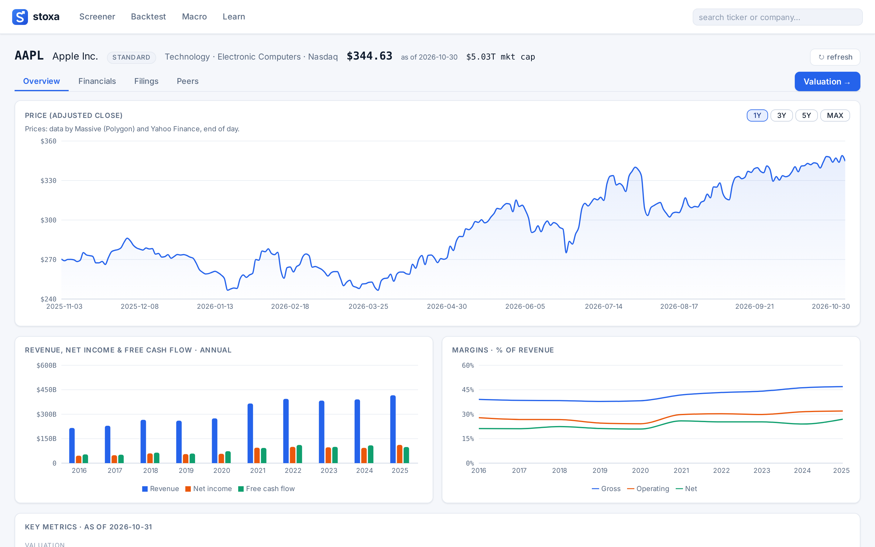
The header shows the ticker, name, company type (standard, financial or REIT, which decides which models apply), sector and industry, the last price with its date, and market cap. The Overview tab has the price chart (1Y, 3Y, 5Y, MAX), a decade of revenue, net income and free cash flow, the margin history, and a grid of Key metrics stamped with their as-of date.

Check the numbers behind the numbers

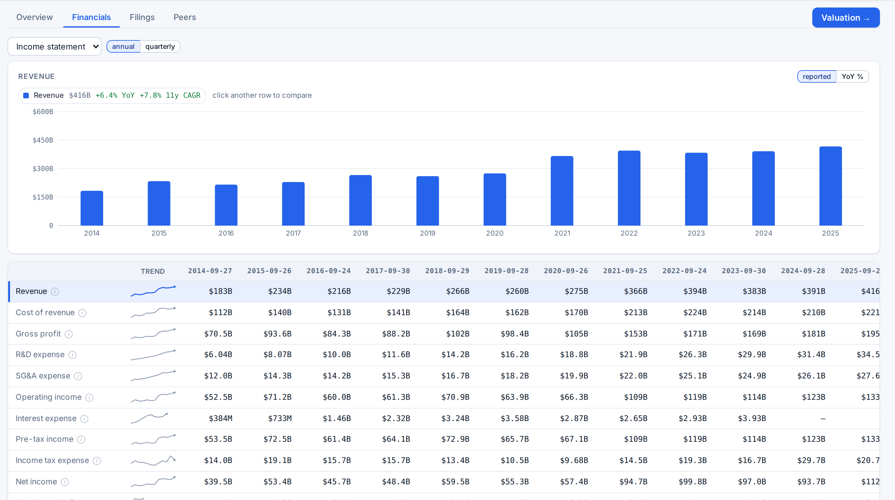
Open Financials to see the income statement, balance sheet or cash flow statement, switching between annual and quarterly. Click any row to chart it; click more rows to compare them on the same chart.

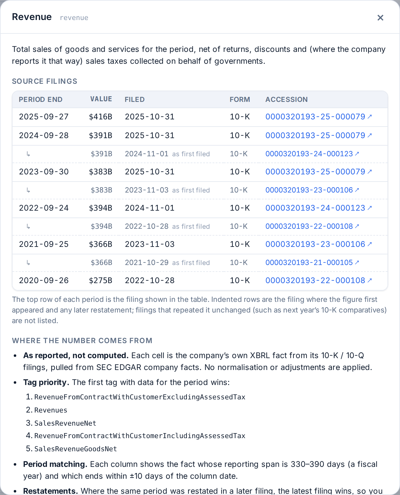
The small i next to each line item (“How is this calculated?”) opens a panel listing the source filings for every period: the value, the date it was filed, the form, and the accession number linking to the filing on SEC EDGAR. Indented rows show where a figure first appeared and whether a later filing restated it. This is the point-in-time record the valuation and the backtester read from. The Filings and Peers tabs list every filing and the companies in the same industry group.

Open the valuation workbench

Click Valuation → on the company page. The workbench opens with defaults derived from the company’s own history: assumptions on the left, results on the right, saved scenarios across the top. Nothing needs to be pressed; the valuation recomputes automatically a moment after you change any input.

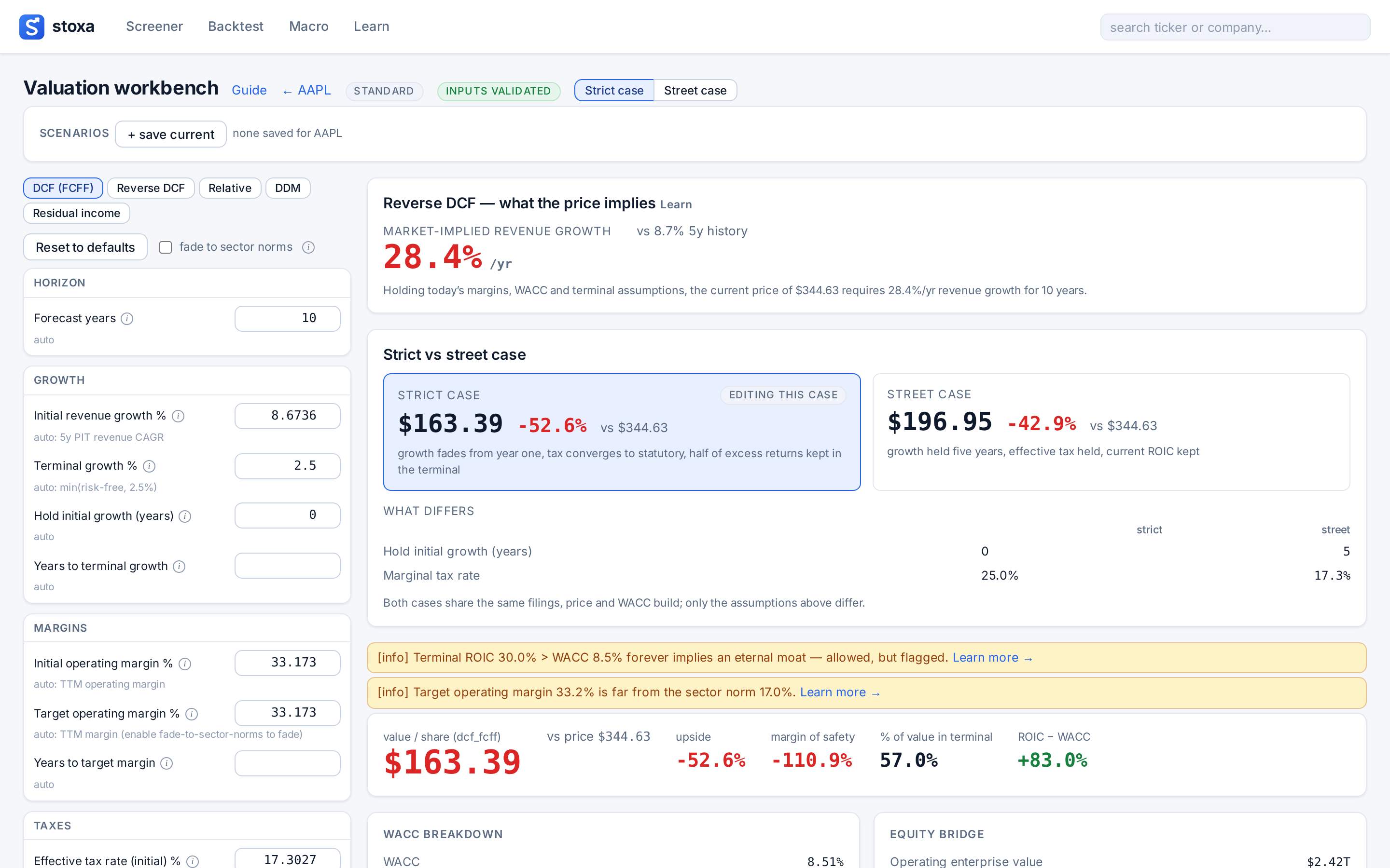
The header badges matter. inputs validated means every data check passed. A cyclical badge means margins default to a mid-cycle average rather than the latest twelve months. When macro data is available, a macro: line summarises the regime as it was known on the valuation date (yield-curve state, CPI, unemployment), with a link to the Macro page.

Heed the data-quality banner

If the inputs fail a plausibility check, a banner sits above the results. Input data has warnings can be expanded with show N checks to read each one in plain language; the red Input data failed validation banner means the valuation should be treated as unreliable until the data is fixed.

The banner is about the data. Problems with your assumptions are flagged separately as warnings in the results; see Guardrails.

Choose a model and a preset

The buttons at the top of the assumptions panel pick the model: DCF (FCFF), Reverse DCF, Relative, DDM and Residual income. Models that do not suit the company are greyed out with the reason on hover; a bank, for example, cannot be valued on free cash flow to the firm. Start with the DCF; use the dividend, residual income and relative models as cross-checks.

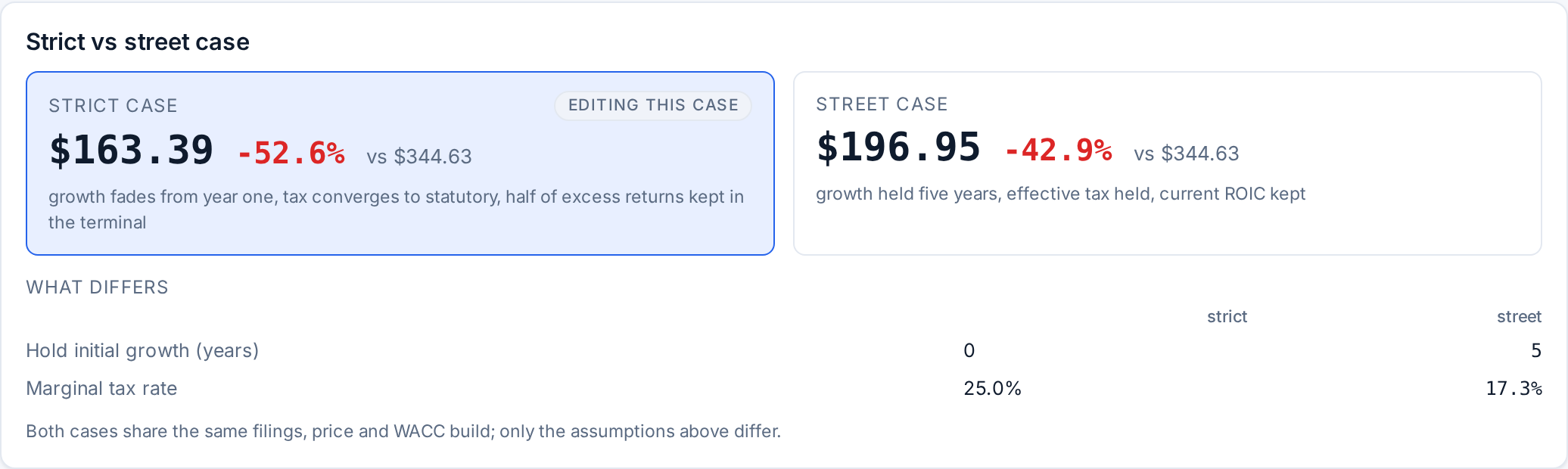
The Strict case / Street case toggle in the header switches the default assumptions. Strict fades growth from year one, moves the tax rate to statutory and keeps half of excess returns in the terminal. Street holds growth for five years, keeps the effective tax rate and the current return on capital, which is closer to typical sell-side numbers.

Edit the assumptions

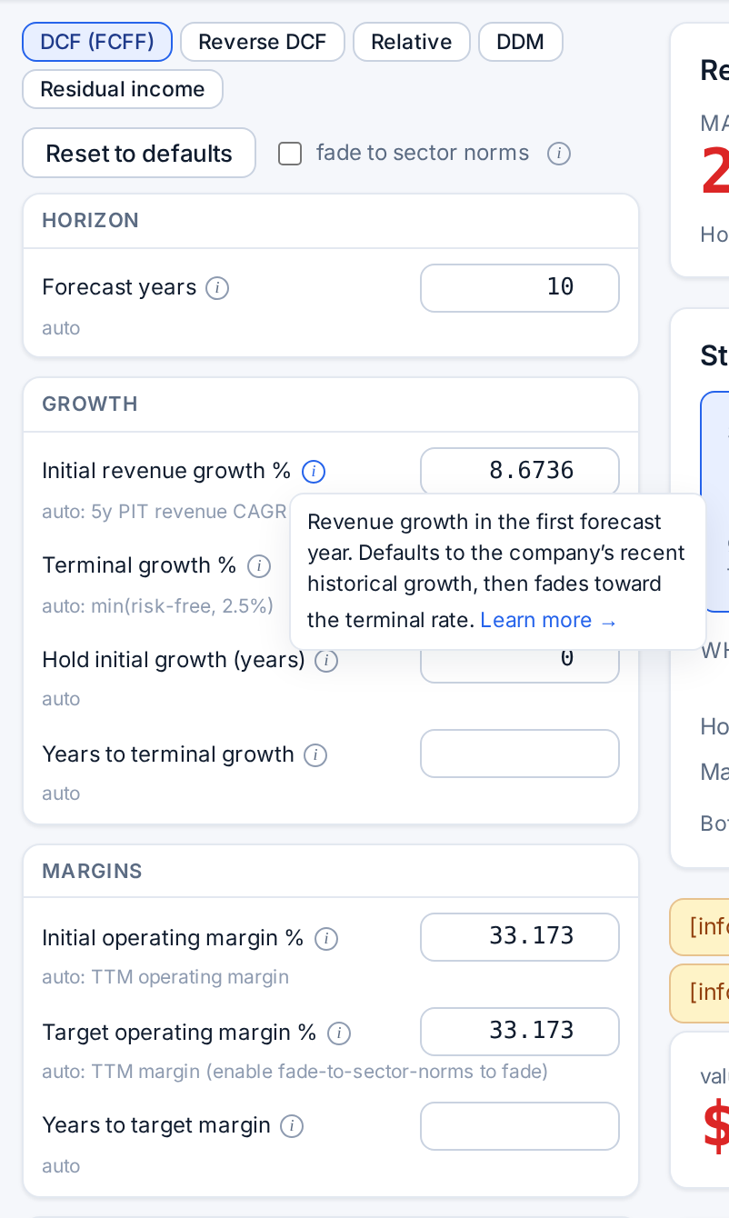
Assumptions are grouped as Horizon, Growth, Margins, Taxes, Reinvestment, WACC and Terminal value. Under each field a grey hint says where the default came from, such as “auto: 5y PIT revenue CAGR”. Percentages are typed as percentages.

Hover or focus the i next to a field for a plain-language explanation and a Learn more → link to the theory page for that input: growth and margin paths, reinvestment, WACC, or terminal value.

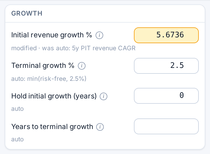
An edited field is highlighted and its hint changes to “modified · was …”, so you can always see which numbers are yours. Reset to defaults puts everything back. fade to sector norms moves the target margin and sales-to-capital ratio toward the sector averages. WACC can be auto (built from risk-free rate, equity risk premium, beta and cost of debt) or manual.

Read the results

The results panel shows value / share next to the price, the upside, the margin of safety, the % of value in terminal and the ROIC − WACC spread. Below them, the WACC breakdown and the Equity bridge show how enterprise value becomes value per share (see From enterprise value to a share price).

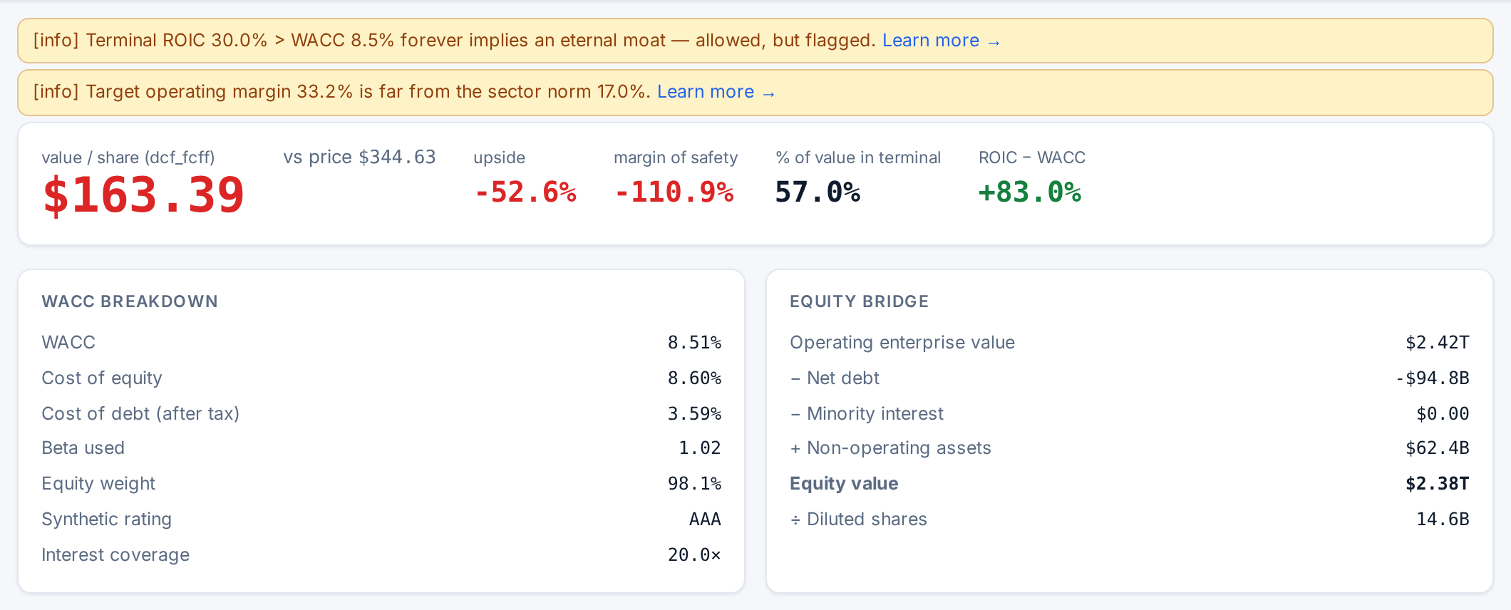
Yellow lines above the result are guardrail warnings: an assumption that is allowed but deserves a second look, such as a terminal return on capital far above the cost of capital, or a margin far from the sector norm. Each links to the reasoning. When most of the value sits in the terminal, the result depends mostly on your terminal assumptions. The Projection chart and table further down show revenue, EBIT, NOPAT, reinvestment, FCFF and present value for every forecast year.

Compare the strict and street cases

With the DCF selected, the Strict vs street case card values the company under both presets’ default assumptions side by side. The what differs table lists every assumption that differs between them, so you can see exactly where the gap comes from. Click a tile to switch the workbench to that case; the one you are editing is marked editing this case.

See what the price implies

The Reverse DCF — what the price implies panel, shown for the DCF and Reverse DCF models, turns the question around. Holding your margins, WACC and terminal assumptions, it solves for the revenue growth the current price requires, and compares it with the company’s five-year history. Red means the market expects clearly more than history delivered; green means less.

Often this is the more useful number: it is easier to judge whether 28% a year for ten years is plausible than to defend a single value. More in Reverse DCF.

Save scenarios

In the Scenarios bar, + save current stores the current assumptions under a name and shows the resulting value per share. Click a scenario to load it back, or ✕ to delete it. Only the assumptions are stored, so a saved scenario re-runs against the latest filings and price when you load it.

Run a sensitivity table

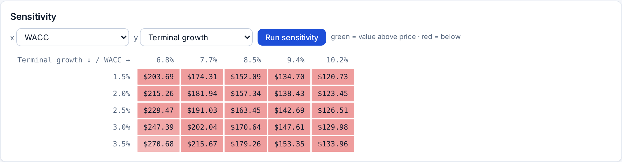
In Sensitivity, choose two inputs for the x and y axes from WACC, Terminal growth, Initial revenue growth and Target operating margin, then Run sensitivity. The grid revalues the company at five values of each around your current assumptions. Green cells are above the current price, red cells below.

Run a Monte Carlo simulation

In Monte Carlo, + add distribution (up to three) and give each input a normal, triangular or uniform distribution. Values here are fractions (0.08 = 8%). Pick n draws and Run simulation.

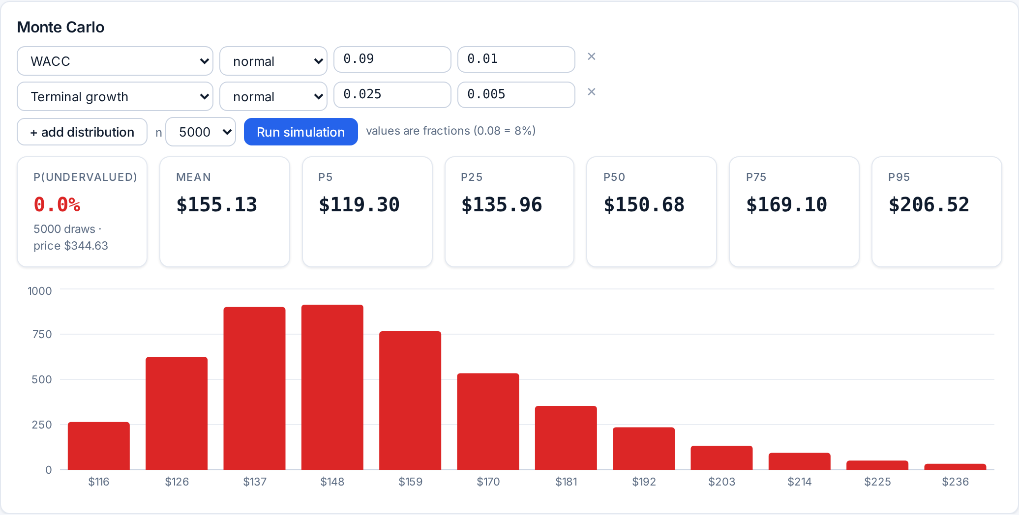
The result is a distribution of values: P(undervalued) is the share of draws above the current price, and P5 to P95 give the range. It answers “how wrong could I be?” better than a single number. See Sensitivity, Monte Carlo and price paths.

Read the output with a margin of safety

A valuation is a structured opinion, not a fact. Read the workbench as a set of answers to “what would have to be true?”: the value under your assumptions, the growth the price implies, the cases that disagree, and how wide the distribution is. In the Apple example the strict model puts value well below the price, while the reverse DCF says the price needs growth far above history. Those are two views of the same gap, and the question for you is which assumptions you believe.

Graham’s margin of safety is the discount to your own estimate you insist on before acting, because every input is uncertain. The wider the sensitivity grid and the Monte Carlo range, the wider that margin should be. Nothing in Stoxa is a recommendation; more in Value versus price.

Everything above is also available programmatically: the Stoxa SDK and REST API expose defaults, valuation runs, reverse DCF, sensitivity and Monte Carlo for scripts and agents. See Stoxa for developers.